DeepSeek只是挖了个坑，还不是掘墓人，但中初级程序员是爬不出来了

在我们的《因子分析与机器学习策略》课程中，提供了从2005年到2023年，长达18年的日线数据（共1100多万条记录）供学员进行因子挖掘与验证。最初，我们是通过functools中的lru_cache装饰器，将数据缓存到内存中的。这样一来，除了首次调用时时间会略长（比如，5秒左右）外，此后的调用都是毫秒级的。

问题的提出

但这样也带来一个问题，就是内存占用太大。一次因子分析课程可能会占用5G以上。由于Jupyterlab没有自动关闭idle kernel的能力（这一点在google Colab和kaggle中都有），我们的内存很快就不够用了。

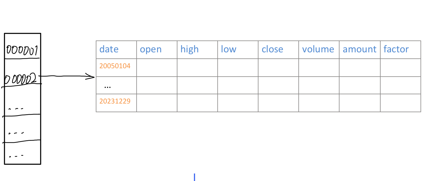
我们的数据是以字典的方式组织，并保存在磁盘上的：

每支股票的键值是股票代码，对应值则是一个Numpy structured array。这样的数据结构看上去比较独特，不过我们稍后就能看到这样组织的原因。

在进行因子分析之前，用户可能会通过指定universe，以及起止时间来加载行情数据。所谓Universe，就是指一个股票池。用户可能有给定的证券列表，也可能只想指定universe的规模；起止时间用来切换观察的时间窗口，这可能是出于性能的考虑（最初进行程序调试时，只需要用一小段行情数据；调试完成后则需要用全部数据进行回测，或者分段观察）。

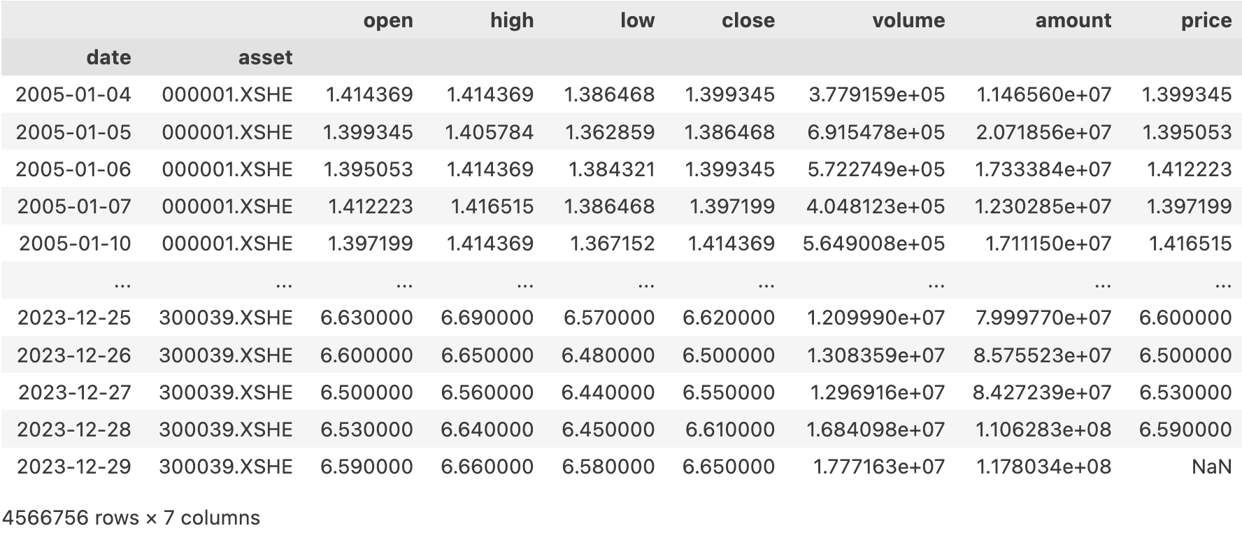
最终，它要返回一个DataFrame，以date和asset（即股票代码）为双重索引，包含了OHLC，volume等列，并且这些列要根据end进行前复权（这种复权方式称为动态前复权）。此外，还将包含一个amount列，这一列则无须复权。

因此，这个函数的签名是：

def load_bars(start_date:datetime.date, 
              end_date:datetime.date, 
              universe: Tuple[str]|int = 500)->pd.DataFrame:
    pass

学员的学习过程是阅读我们的notebook文档，并尝试单元格中的代码，也可能修改这些代码再运行。因此，这是一个交互式的操作，一般来说，只要用户的等待时间不超过3秒，都是可以接受的。如果响应速度低于1秒，则可以认为是理想的。

去掉缓存后，最初的一个实现的运行速度大致是5秒：

start = datetime.date(2023, 12,1)
end = datetime.date(2023, 12,31)
%time load_bars(start, end, 2000)

后面的测试将使用现样的参数。

当然，如果使用更大的universe，则时间还会加长。

由于这个结果超过了3秒，所以，希望能对代码进行一些优化。性能优化是编程中比较有难度的例子，因为它涉及到对程序运行原理的理解，涉及到对多个技术栈的掌握。在这个过程中我探索了Deep Seek R1的能力边界，可供大家参考。

最初的方案

最初的代码如下：

def load_bars_v1(
    start: datetime.date, end: datetime.date, universe: Tuple[str]|int = 500
)->pd.DataFrame:

    if barss is None:
        with open(os.path.join(data_home, "bars_1d_2005_2023.pkl"), "rb") as f:
            barss = pickle.load(f)

    keys = list(barss.keys())
    if isinstance(universe, int):
        if universe == -1:
            selected_keys = keys
        else:
            selected_keys = random.sample(keys, min(universe, len(keys)))
            try:
                pos = selected_keys.index("000001.XSHE")
                swp = selected_keys[0]
                selected_keys[0] = "000001.XSHE"
                selected_keys[pos] = swp
            except ValueError:
                selected_keys[0] = "000001.XSHE"

    else:
        selected_keys = universe

    dfs = []
    for symbol in selected_keys:
        qry = "frame >= @start & frame <= @end"
        df = pd.DataFrame(barss[symbol]).assign(asset=symbol).query(qry)

        if len(df) == 0:
            logger.debug("no bars for %s from %s to %s", symbol, start, end)
            continue
        # 前复权
        last = df.iloc[-1]["factor"]
        adjust_factor = df["factor"] / last
        adjust = ["open", "high", "low", "close", "volume"]
        df.loc[:, adjust] = df.loc[:, adjust].multiply(adjust_factor, axis="index")

        dfs.append(df)

    df = pd.concat(dfs, ignore_index=True)
    df.set_index(["frame", "asset"], inplace=True)
    df.index.names = ["date", "asset"]
    df.drop("factor", axis=1, inplace=True)
    df["price"] = df["open"].shift(-1)
    return df

代码已进行了相当的优化（其中部分也基于AI建议）。比如，将数据保存为字典，先按universe进行筛选，再拼接为dataframe，而不是将所有数据保存为dataframe，通过pandas来按universe进行筛选（将花费数倍时间）。

此外，在进行前复权时，它使用了multiply方法，从而可以一次对多个列进行前复权操作，这一建议正是AI给出来的。

但是，代码中还存在一个for loop，如果消除了这个循环，是否能进一步提升速度呢？

下面，我就使用Deep Seek R1进行尝试。

这是第一轮的prompt:

Quote

我有一个dataframe，以date和asset为联合索引，有open, high, low, close, volume, amount和factor等列。其中factor是复权因子。
现在，要对该数据结构实现以下功能：
1. 筛选出asset 在 selected_symbols列表中，date在[start, end]中的记录 2. 对这些记录，按asset进行分组，然后对 open, high, low, close, volume进行前复权。 3. 结果用dataframe返回，索引仍为date/asset，列为复权后的open, high,low, close, volume字段，以及未处理的amount。
请分别给出基于pandas， pyarrow, polars, duckdb的实现，并建议性能最优的一个。

Deep Seek的思考过程很长，这里略过了。我们直接看它的答案。磁盘读写对速度的影响并不大，所以，我们先把数据从磁盘中加载出来，保存到barss中：

with open(os.path.join(data_home, "bars_1d_2005_2023.pkl"), "rb") as f:
    data = pickle.load(f)

dfs = []
for symbol, bars in data.items():
    df = pd.DataFrame(bars)
    df["asset"] = symbol
    df = df.rename(columns={"frame": "date"})
    dfs.append(df)

barss = pd.concat(dfs,ignore_index=True).set_index(["date", "asset"]).sort_index()
print(len(barss))

# 定义一个一致的universe，便于比较
universe = barss.index.get_level_values("asset").unique().tolist()

以下的代码都出自于 Deep Seek。我们让它对最耗时的筛选和复权部分给出方案：

基于Pandas的实现

def adjust_pandas(df, selected_symbols, start, end):
    # 筛选数据
    idx = pd.IndexSlice
    filtered = df.loc[idx[start:end, selected_symbols], :]

    # 按 asset 分组计算最后复权因子
    grouped = filtered.groupby('asset', group_keys=False)
    last_factor = grouped['factor'].transform('last')

    # 计算调整比例
    ratio = filtered['factor'] / last_factor

    # 计算复权后字段
    adjusted = filtered.assign(
        open   = filtered['open'] * ratio,
        high   = filtered['high'] * ratio,
        low    = filtered['low'] * ratio,
        close  = filtered['close'] * ratio,
        volume = filtered['volume'] * (last_factor / filtered['factor'])
    )

    # 选择最终列并保持索引
    return adjusted[['open', 'high', 'low', 'close', 'volume', 'amount']]

%time adjust_pandas(barss, universe, start, end)
adjust_pandas(barss, universe, start, end)

尽管我对Pandas很熟悉了，但仍有一些API是不知道的，比如transform。但运用正确的API，恰恰是 Python中提升性能的关键一招。

这个版本的平均运行时长是7秒。说明pandas的筛选确实很慢。

我们略过pyarrow的版本。pyarrow版本的运行时间大致是3.7秒左右。比原始版本只略有进步。这里也看出python 3.11中，for loop的运行速度已经很快了。

基于Polars的实现

这是它给出的polars的版本：

import polars as pl

def adjust_polars(df, selected_symbols, start, end):
    # 筛选数据
    filtered = df.filter(
        (pl.col("date").is_between(start, end)) &
        (pl.col("asset").is_in(selected_symbols))
    )

    # 计算最后复权因子和调整比例
    adjusted = filtered.with_columns(
        last_factor = pl.col("factor").last().over("asset")
    ).with_columns(
        ratio = pl.col("factor") / pl.col("last_factor"),
        volume_ratio = pl.col("last_factor") / pl.col("factor")
    ).with_columns(
        open   = pl.col("open") * pl.col("ratio"),
        high   = pl.col("high") * pl.col("ratio"),
        low    = pl.col("low") * pl.col("ratio"),
        close  = pl.col("close") * pl.col("ratio"),
        volume = pl.col("volume") * pl.col("volume_ratio")
    )

    # 选择最终列
    return adjusted.select(["date", "asset", "open", "high", "low", "close", "volume", "amount"])

adjust_polars(barss, universe, start, end)

之前我并不熟悉Polars，Deep Seek一下子扩展了我的能力边界。如果我要通过自学，然后来实现这部分功能，我不知道要多久才能发现.over这个API，因为这是 Polars 独有的一个窗口运算API，我无法把知识从我熟悉的Pandas中迁移过来。

但是，这个版本有一个错误：它没有遵从我给的数据格式，而是把barss当成了一个有asset和date列的polars DataFrame。通过使用通义灵码，修正了此错误，修正后的代码如下：

%time adjust_polars(pl.from_pandas(barss.reset_index()), universe, start, end)

得到的运行速度是1.01秒，已很接近我们要求的理想速度了。

基于DuckDB的实现

现在，我们来看它给出的duckdb的版本：

import duckdb

def adjust_duckdb(df, selected_symbols, start, end):
    query = f"""
    SELECT 
        date, asset,
        open * (factor / last_factor) AS open,
        high * (factor / last_factor) AS high,
        low * (factor / last_factor) AS low,
        close * (factor / last_factor) AS close,
        volume * (last_factor / factor) AS volume,
        amount
    FROM (
        SELECT 
            *,
            LAST_VALUE(factor) OVER (
                PARTITION BY asset 
                ORDER BY date 
                ROWS BETWEEN UNBOUNDED PRECEDING AND UNBOUNDED FOLLOWING
            ) AS last_factor
        FROM df
        WHERE 
            asset IN ({','.join([f"'{s}'" for s in selected_symbols])})
            AND date BETWEEN '{start}' AND '{end}'
    )
    """
    return duckdb.query(query).to_df()

adjust_duckdb(barss, universe, start, end)

这里也会出现一个类似的错误，即查询语句需要df中存在asset, date列，但它们却出现在索引中。我们略作修正即可运行：

%time adjust_duckdb(barss.reset_index(), universe, start, end)

最终运行速度是1.21秒，在这个例子中略慢于polars，在所有方案中排在第二（在另一台机器，使用机械阵列硬盘时，更强的CPU时， duckdb更快）。但是，duckdb方案在数据规模上可能更有优势，即，如果数据集再大一到两个量级，它很可能超过polars。

在polars与duckdb中，需要的都是扁平结果的数据结构（即asset/date不作为索引，而是作为列字段存在），因此，我们可以考虑将数据结构进行重构，使用apache parquet格式写入到磁盘中，这样可以保存整个方案耗时仍保持在1秒左右。

终极咒语：急急如律令

Info

据说急急如律令要翻译成为 quickly, quickly, biu biu biu 😁

在前面，我们代替Deep Seek做了很多思考，是因为担心它对代码的最终执行速度没有sense。现在，我们试一下，直接抛出最终问题，看看会如何：

Quote

我有一个dataframe，以date和asset为联合索引，有open, high, low, close, volume, amount和factor等列。其中factor是复权因子。

现在，要对该数据结构实现以下功能：

1. 筛选出asset 在 selected_symbols列表中，date在[start, end]中的记录
2. 对这些记录，按asset进行分组，然后对 open, high, low, close, volume进行前复权。
3. 结果用dataframe返回，索引仍为date/asset，列为复权后的open, high,low, close, volume字段，以及未处理的amount。

输入数据是1000万条以上，时间跨度是2005年到2023年，到2023年底，大约有5000支股票。输出结果将包含2000支股票的2005年到2023年的数据。请给出基于python，能在1秒左右实现上述功能的方案。

这一次，我们只要求技术方案限定在Python领域内，给了Deep Seek极大的发挥空间。

Deep Seek不仅给出了代码，还给出了『评测报告』，认为它给出的方案，能在某个CPU+内存组合上达到我们要求的速度。

Deep Seek认为，对于千万条记录级别的数据集，必须使用像parallel pandas这样的库来进行并行化才能达成目标。事实上这个认知是错误的。

这一次Deep Seek给出的代码可运行度不高，我们没法验证基于并行化之后，速度是不是真的更快了。不过，令人印象深刻的是，它还给出了一个performance benchmark。这是它自己GAN出来的，还是真有人做过类似的测试，或者是从类似的规模推导出来的，就不得而知了。

重要的是，在给了Deek Seek更大的自由发挥空间之后，它找出了之前在筛选时，性能糟糕的重要原因： asset是字符串类型！

在海量记录中进行字符串搜索是相当慢的。在pandas中，我们可以将整数转换为category类型，此后的筛选就快很多了：

import pyarrow as pa
import pyarrow.parquet as pq

data_home = os.path.expanduser(data_home)
origin_data_file = os.path.join(data_home, "bars_1d_2005_2023.pkl")
with open(origin_data_file, 'rb') as f:
    data = pickle.load(f)

dfs = []
for symbol, bars in data.items():
    df = pd.DataFrame(bars)
    df["asset"] = symbol
    df = df.rename(columns={"frame": "date"})
    dfs.append(df)

barss = pd.concat(dfs,ignore_index=True)
barss['asset'] = barss['asset'].astype('category')
print(len(barss))

table = pa.Table.from_pandas(barss)

parquet_file_path = "/tmp/bars_1d_2005_2023_category.parquet"

with open(parquet_file_path, 'wb') as f:
    pq.write_table(table, f)

现在，我们再来看polars或者duckdb的方案的速度：

import polars as pl

def adjust_polars(df, selected_symbols, start, end):
    # 筛选数据
    filtered = df.filter(
        (pl.col("date").is_between(start, end)) &
        (pl.col("asset").is_in(selected_symbols))
    )

    # 计算最后复权因子和调整比例
    adjusted = filtered.with_columns(
        last_factor = pl.col("factor").last().over("asset")
    ).with_columns(
        ratio = pl.col("factor") / pl.col("last_factor"),
        volume_ratio = pl.col("last_factor") / pl.col("factor")
    ).with_columns(
        open   = pl.col("open") * pl.col("ratio"),
        high   = pl.col("high") * pl.col("ratio"),
        low    = pl.col("low") * pl.col("ratio"),
        close  = pl.col("close") * pl.col("ratio"),
        volume = pl.col("volume") * pl.col("volume_ratio")
    )

    # 选择最终列
    return adjusted.select([pl.col("date"), pl.col("asset"), pl.col("open"), pl.col("high"), pl.col("low"), pl.col("close"), pl.col("volume"), pl.col("amount")])

# 示例调用
start = datetime.date(2005, 1, 1)
end = datetime.date(2023, 12, 31)

barss = pl.read_parquet("/tmp/bars_1d_2005_2023_category.parquet")

universe = random.sample(barss['asset'].unique().to_list(), 2000)

%time adjust_polars(barss, universe, start, end)

结果是只需要91ms，令人印象深刻。duckdb的方案需要390ms，可能是因为我们需要在Python域拼接大量的selected_symbols字符串的原因。

借助 Deep Seek，我们把一个需要5秒左右的操作，加速到了0.1秒，速度提升了50倍。

本文测试都在一台mac m1机器上运行，RAM是16GB。当运行在其它机器上，因CPU，RAM及硬盘类型不同，数据表现甚至排名都会有所不同_。

结论

这次探索中，仅从解决问题的能力上看，Deep Seek、通义和豆包都相当于中级程序员，即能够较好地完成一个小模块的功能性需求，它情绪稳定，细微之处的代码质量更高。

当我们直接要求给出某个数据集下，能达到指定响应速度的Python方案时，Deep Seek有点用力过猛。从结果上看，如果我们通过单机、单线程就能达到91ms左右的响应速度，那么它给出的多进程方案，很可能是要劣于这个结果的。Deep Seek只是遵循了常见的优化思路，但它没有通过实际测试来修正自己的方案。

这说明，它们还无法完全替代人类程序员，特别是高级程序员：对于AI给出的结果，我们仍然需要验证、优化甚至是推动AI向前进，而这刚好是高级程序员才能做到的事情。

但这也仅仅是因为AI还不能四处走动的原因。因为这个原因，它不能像人类一样，知道自己有哪些测试环境可供方案验证，从而找出具体环境下的最优方案。

在铁皮机箱以内，它是森林之王，人类无法与之较量。但就像人不能拔着自己的头发离开地球一样，它的能力，也暂时被封印在铁皮机箱之内。但是，一旦它学会了拔插头，开电源，高级程序员的职业终点就不再是35岁，而是AI获得自己的莲花肉身之时。

至于初中级程序员，目前看是真不需要了。1万元的底薪，加上社保，这能买多少token? 2025年的毕业生，怎么办？