上期重要日历提示本周为超级央行周，叠加美股科技股年报，风浪比较大。果然，这周外围股市受到严重冲击。英特尔更是一天下跌超 26%。

本周要闻回顾

• 美国 7 月非农数据爆冷，萨姆规则被触发，美联储未就降息做出决定
• 日本央行加息，引爆全球股市重挫，原油、美元大跌，人民币大涨近千点！
• 金融圈打虎！董国群、陈小澎等被查
• 英伟达 Blackwell 芯片缺陷导致量产推迟

下周看点

• 周一财新发布 PMI，周五统计局发布 CPI/PPI。
• 减肥双雄诺和诺德与礼来均将于下周公布季报
• 工程机械巨头卡特彼勒和娱乐巨头迪士尼分别将于下周二和周三公布财报

本周精选

• 二阶导因子跑出 Alpha 61.5%!（公众号付费文章）
• TradeGPT! 快来用 ChatGPT 生成交易策略！
• Awesome! 资产新闻情感分析新工具
• 你们都是在哪儿下载论文的？附两个网站，速度！

---

要闻回顾

• 美国 7 月非农数据爆冷，萨姆规则被触发，美联储未就降息做出决定
  美劳工部数据称，7 月美国新增就业 11.4 万，薪资增速回落至 3.6%，刷新近三年低点。同时，失业率则由 4.1%上升到 4.3%，已触发预示衰退的萨姆规则。
  在上周的美联储议息会议上，美联储决定将基准利率维持在 5.25%~5.50%的区间内。由于美联储在 8 月和 10 月没有常规议息会议，因此，9 月份的议息会议将十分关键。
  鲍威尔称，如果美国经济按照预期走势发展，美联储最早可能在 9 月份降息。关于萨姆规则，鲍威尔称知道萨姆规则，称其为统计规律。 不过也有分析认为，7 月非农数据受季节性飓风影响。
  
• 日本央行加息，叠加美股科技股年报和非农数据不及预期，引爆全球股市重挫。日经周五重挫 5.81%，纳指下跌 2.43%。英特尔暴跌逾 26%，并且预计第三季度收入低于预期，将裁员 1.5 万人。其它大幅下跌科技股还有亚马逊（-8.78%）、阿斯麦（-8.41%）。原油周五下跌 3.41%，美元对六种主要货币指数下跌 1.15%，人民币上涨 873 点。
• 金融圈打虎！原上交所副总董国群、证监会深圳监管局原党委书记、局长陈小澎等被查。海通证券公告，公司副总经理姜诚君申请辞职。
• 英伟达 Blackwell 芯片缺陷导致量产推迟，涉及数百亿美元芯片订单。同时，英伟达还面临美国司法部反垄断调查。
• 因全球化工龙头巴斯夫在德国的工厂突发爆炸，维生素 A 报价 2 天飙升 53%，维生素 E 报价上涨 20%。8月1日晚，巴斯夫（中国）公司对证券时报记者称，何时复产，目前无法评估和判断。

根据财联社、东方财富、证券时报等资讯汇编

---

二阶导因子跑出 ALPHA 61.5%!

这一期，我们将介绍一个二阶导因子。我们将演示二阶导因子的探索优化过程，进一步介绍因子分析的原理，包括：

1. 如何让 Alphalens 使用我们指定的分层
2. 二阶导动量因子的数学原理
3. By quantiles or By bins, 分层究竟意味着什么

最后，我们在 A 股 40%的抽样中，得到最近半年二阶导因子的最佳参数是 5 天。在此参数下，年化 Alpha 分别是 38.4%（多空）和 61.5%（单边做多）， beta 为-0.12，即收益独立于市场。

上一期我们检视了斜率因子。本质上，斜率因子是一阶导动量因子。比如，以如下方式生成的数组，它的斜率和一阶导是相等的：

from scipy.stats import linregress

slope = 0.2
x = np.arange(10)
y = slope * x + 1

d1 = np.diff(y).mean()

# 如果我们通过线性回归来求斜率
alpha, beta, *_ = linregress(x, y)

print(f"slope is {slope:.1f}")
print(f"first derivative is {d1:.1f}")
print(f"slope by linear regression is {alpha:.1f}")

三项输出都是 0.2。如果我们对价格序列求二阶导作为因子，它会对未来趋势有预测作用吗？我们先看结果，再来讨论背后的原理。

二阶导动量因子检验

下面这段代码可以生成一个二阶导动量因子。

---

def d2_factor(close: NDArray, win: int = 10) -> NDArray:
    n = len(close)

    d1 = close[1:]/close[:-1] - 1
    d2 = d1[1:] - d1[:-1]

    factor = move_mean(d2, win)
    # 进行左填充，使之与输入等长
    factor = np.pad(factor, (n-len(factor), 0), ...)

    return factor

注意我们用close[1:]/close[:-1]-1代替了通常意义上的一阶导，以起到某种标准化的作用。如果我们不这样做，那么高价股的因子将永远大于低价股的因子，从而永远有更高的因子暴露。

因子本身的参数是win，表示我们是在多长的时间段内计算的二阶导。

然后我们通过 Alphalens 来进行因子检验。第一次调用 Alphalens，我们按 quantiles 分层，分层数为 10。

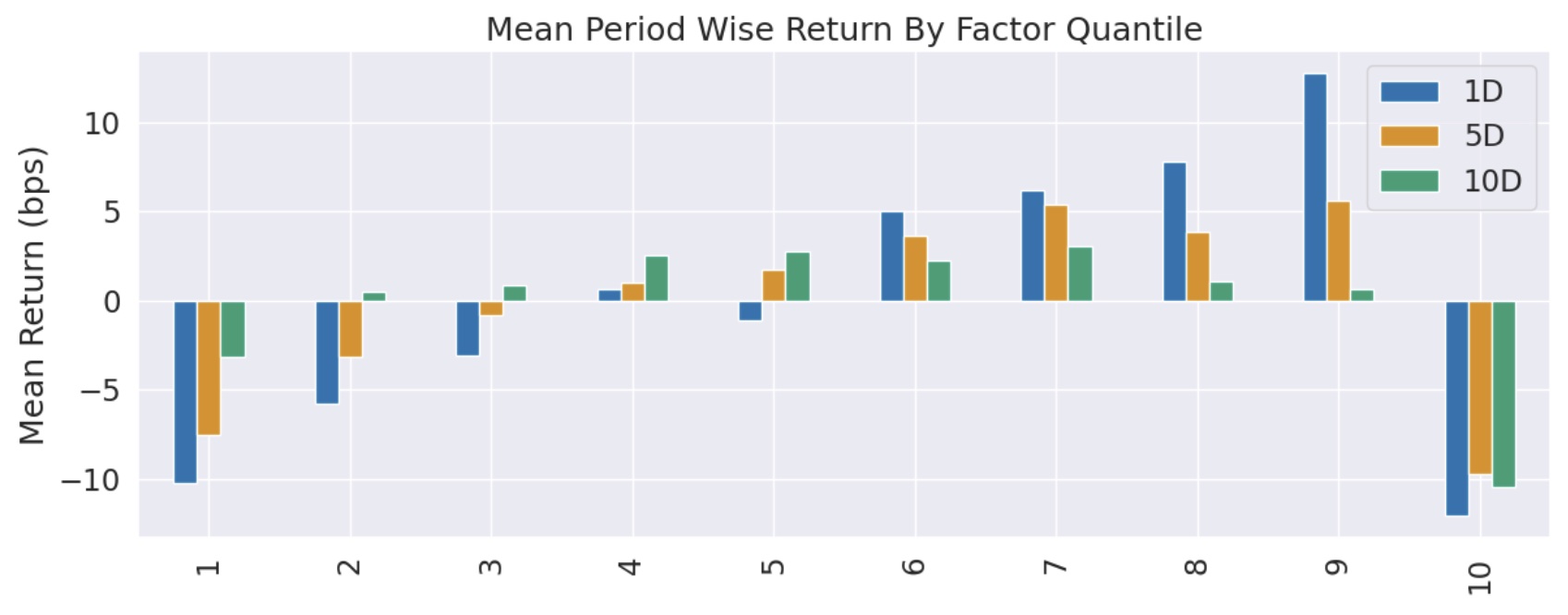
从分层图来看，继续进行收益分析是没有意义的，我们必须先进行优化。

第一次调优

考虑到做多收益在第 8 层达到最大值，所以，我们考虑 drop 掉第 9 层和第 10 层后进行分析，看看结果如何。

通过 Alphalens 进行分析中，一般有三个步骤：

---

1. 构造因子。
2. 数据预处理，一般是通过调用 get_clean_factor_and_forward_returns 来实现的。
3. 调用 create_full_tearsheet 来执行因子检验并输出报表。它的输入是第 2 步中的输出。

Alphalens 是在第二步实现的分层。然后它将第二步的输出，用作第 3 步的输入。

所以，我们可以在拿到第 2 步的输出之后，drop 掉第 9 层和第 10 层，然后调用 create_full_tearsheet 来进行收益分析。这样，在 Alphalens 看来，top 分层就是第 8 层，所有的分析都是在这个基础上进行。

根据 Alphalens 的官方文档，这样做是允许的。

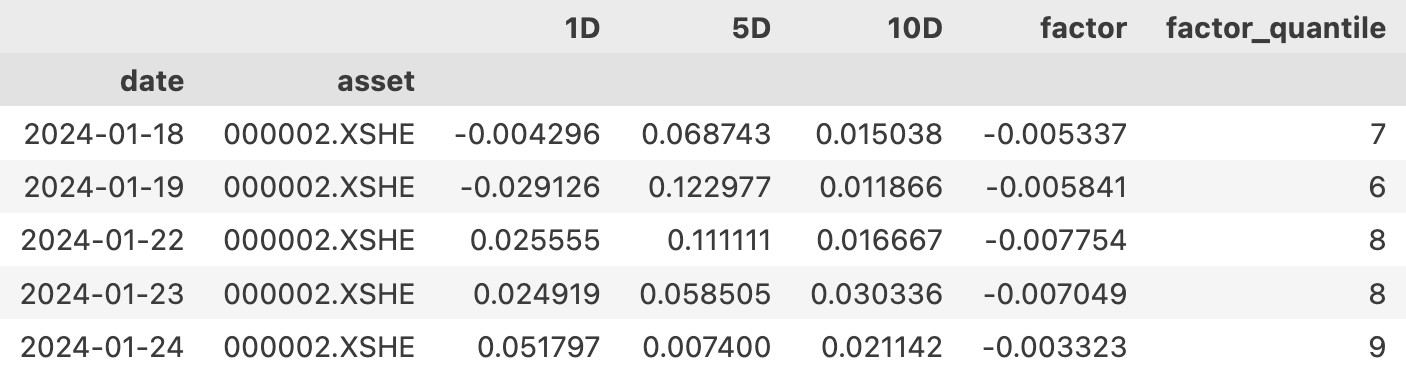
第 2 步输出的是一个 DataFrame，它的格式如下：

所以，要 drop 掉第 9 层和第 10 层，可以这样做：

factor_data = factor_data[factor_data.factor_quantile <= 8]

Tip

这是本文介绍的第一个技巧。在前面的课程中，为了让 Alphalens 按照我们的意愿，按指定的对空分层进行收益分析，我们使用的是改造因子本身的方法，比这个方法在阶段上更提前一些。两个方法都可以使用，但这里的方法更简单。

---

这一次我们得到了令人满意的分层收益均值图，单调且递增，完全适合进一步进行因子分析。

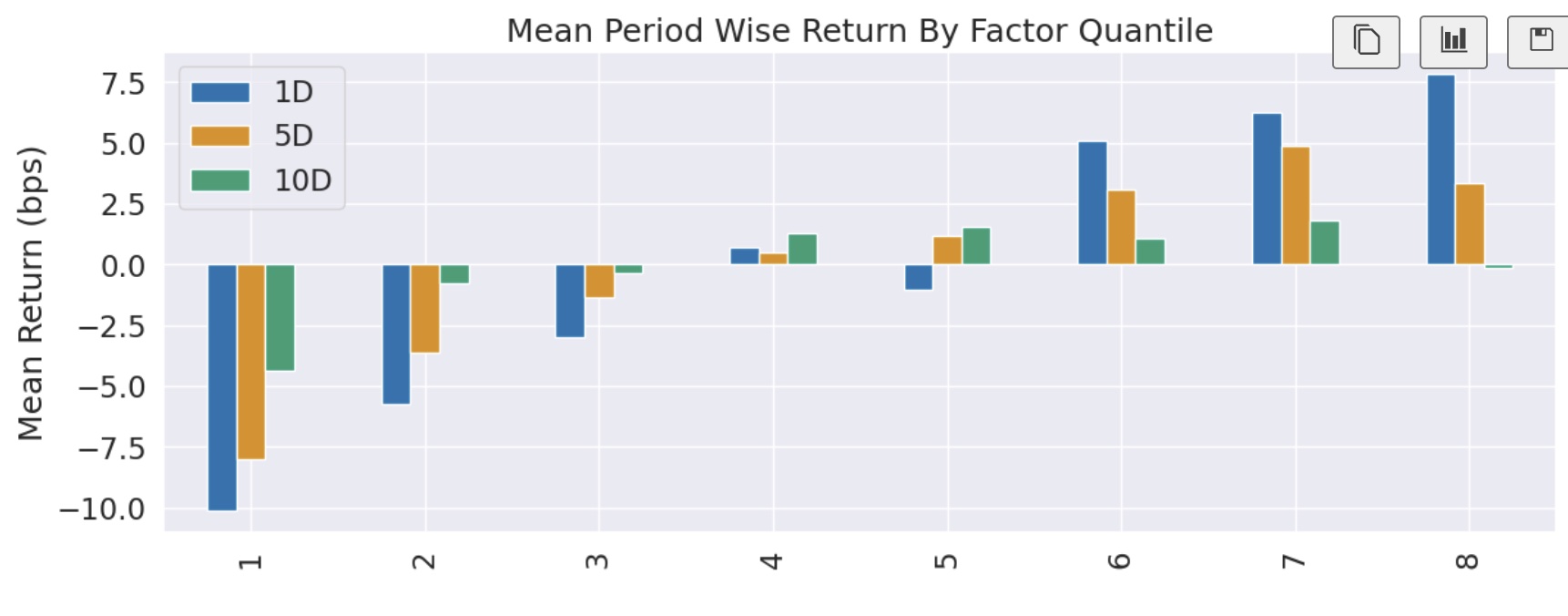
这个图其实基本上就是完全还原了上一个图，只不过缺少第 9 层和第 10 层而已。但是，现在第 8 层就成了 top 分层，这是 Alphalens 在计算多空收益时，将要做多的一层。

Tip

由于我们在实盘交易中也一样可以 drop 掉第 9 层和第 10 层，因此这种操作是合理的。类似的手法，我们在 Alpha101 中也可以看到。

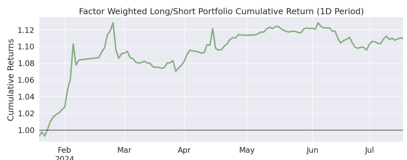
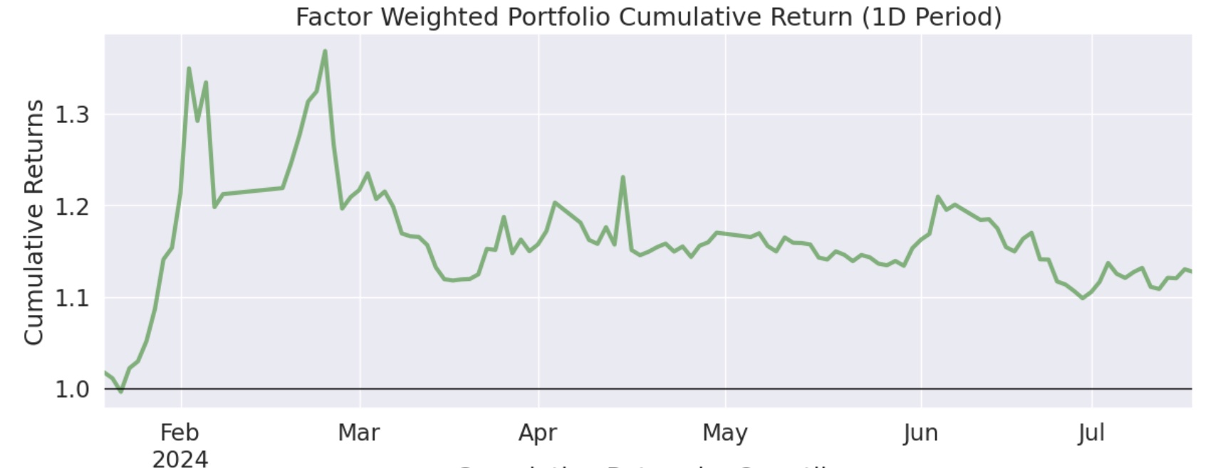
现在我们得到的 Alpha 是 23.2%（1D 年化），Beta 是-0.07，7 个月的累计收益是 11%左右。

纯多的情况

我们在之前的几期里讲过，由于制度因素，并不是所有人都能条件做空。所以我们看看纯做多的情况下，因子表现如何。

这一次，年化 Alpha 只有 17.6%，beta 为-0.6。但 7 个月的累积收益是 15%左右，还略高了一些。

---

条件	Alpha	Beta	累计收益
多空、10	23.2%	-0.07	11%
单多、10	17.6%	-0.60	15%

我们对比一下前后两次的累积收益图，可以发现，多空组合绝对收益低了一些，但平抑风险的能力更强了：

多空组合

单边做多

为什么多空的 Alpha 大于纯多，多空组合的累积收益还低于单边做多？这可能是在对二阶导因子做空的过程中，有一些负面效应。一些强势股，在急杀之后（二阶导为负），往往还会有一个小反弹，如果刚好在小反弹前做空，就会带来损失。

---

寻找最有效的窗口

到目前为止，我们使用的都是 10 天的窗口来计算的二阶导。如果使用其它窗口呢？我们分别测试了 2、4、6、8 天的数据。现在，我们把所有的数据汇总起来：

条件	Alpha	Beta	累计收益
多空、2	30.6%	-0.06	15%
多空、4	35.3%	-0.1	17%
多空、5	38.4%	-0.12	19%
多空、6	37.3%	-0.12	18%
多空、8	32.4%	-0.06	14.8%
多空、10	23.2%	-0.07	11%
单多、10	17.6%	-0.60	15%
单多、5	61.5%	-0.58	37%

看起来在 A 股市场上，二阶导动量因子使用周期为 5 时表现最好。此时如果能构建多空组合，年化 Alpha 是 38.4%，今年以来累计收益是 19%；如果只能构建单多组合，年化 Alpha 是 61.5%，今年以来累计收益是 37%。

回顾一点高中数学

前一期讨论的斜率因子（即一阶导因子）反映的是价格上涨的速度。

那么二阶导因子代表什么呢？

二阶导因子反映的是价格变化的加速度。

---

当一阶导为正，而二阶导为负时，价格将仍然上涨，但趋势减缓，有可能出现变盘。反之亦然。下面的公式显示了一个存在二阶导的函数：

\[ y = a x^2 + b x + c \]

当 a 和 b 分别在 [-1, 0, 0, 1] 和 [10, 10, -10, -10] 之间取值时，我们就得到下面的图形：

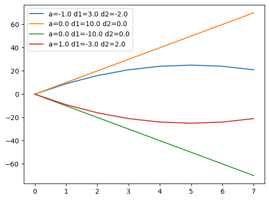
这个图说明，二阶导对证券价格运行的趋势具有修正效应。本来处于上涨趋势的品种，如果二阶导持续为负，它迟早会到达峰顶、然后转为下跌；反之，本来处于下跌趋势的品种，如果二阶导持续为正，它迟早会触及谷底，然后转为上涨。

正因为这样，与一阶导不同，二阶导有能力提前预测价格趋势的变化。它是一种反转动能。

在测试中，表现最好的参数是 5 天。考虑到二阶导需要额外多两个窗口才能计算，因此我们实际上是基于过去 7 天的数据来发出交易信号。

7 天，这是上帝之数。

眼见为实

看到 38%的 Alpha，老实说有点吃惊。

---

这是真的吗？还是说什么地方 Pseudo-Logoi，这位谎言之神悄悄地溜了进来？

尽管可以相信 Alphalens 是品质的保证，但比起一堆统计数字，你可能更愿意相信自己的卡姿兰大眼睛。

所以，我决定把第 8 层的个股走势画出来。绘制方法是，先取出某一天（记为 T0）quantile = 8 的所有标的，然后再取出最近 8 天（截止 T0 为止）的收盘价。在绘图之前，先对收盘价起点归一化到 1。

绘图中，我们共使用了 199 个样本，代表性和稳健性都足够了。

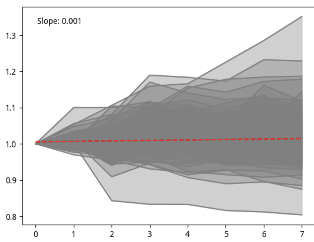
图中的红色线是趋势线，其斜率是 0.001，表明总体上是上涨的；颜色的深浅，代表了样本的分布密度，可以看出，零线上方分布更多一些。

---

我很喜欢从一些股谚中寻找灵感。因为公司底色、市场机制和交易制度的不同，照搬海外股市的做法是行不通的。我们这边博弈的底色更重一点。

按理说，跟二阶导动量因子有关的股谚是黄金坑和圆弧顶，或者 V 反。那么，能直观地画出来在这些标的中，有多少漂亮的黄金坑吗？

很难只用一张图、同一个参数就绘制出来：每个黄金坑的周期、深度和构造阶段等指标都是不一样的。环肥燕瘦，我们很难一笔画尽美人风姿。

By bins, or By quantiles？

在这次测试中，我们一直使用的都是 by quantiles 进行的分层，没有探索 by bins 分层。

by quantiles 是一种排名分层。这是 quantiles 的定义决定的。使用 by bins 方法，我们更关注的是因子值本身的金融含义。

比如，对 RSI 来说，它的值在 0 到 100 之间，大家会认为超过 80 的值是“超买”，低于 20 的值是“超卖”。因此，直接使用因子值是有意义的。

本文没有使用 by quantiles 方法，一方面因子值本身的信号意义可能没那么强：

我们寻找买入或者卖出信号，是根据后面是涨还是跌来验证的。但是，二阶导只能告诉我们趋势的改变方向，并不能立即决定涨跌。

因此，我们可能更应该使用它的排名来做因子，因为资金往往会寻找反转动能最强的标的。

---

Info

题外话：by quantiles 分层用的是排名，有点 Rank IC 的感觉，但计算收益时，又是根据因子值来进行权重分配的，则与 Ranked IC 的方法区别。

通过这些参数以及它们之间的混搭，Alphalens 赋予了我们强大的探索能力。

另一方面，我并不清楚它的最小值、最大值和分布情况，所以在实操上难以给出 bins 数组。这也是没有使用 by bins 的原因。

当然，这并非绝对。也许，有时间的话，也应该探索下 by bins 分层。

如果需要获取全部代码及进行测试，可以通过 公众号付费文章 获得运行环境、代码和数据。

---

TradeGPT! 快来用 CHATGPT 生成交易策略

通过 ChatGPT，我们可以基于宏观经济层面生成一些有用的交易策略。

要有效使用 ChatGPT，我们可以尝试 RISE 提问模型，即 Role, Instructions, Steps and End goal 模型。下面是一个例子：

Role: Assume the role of a world-class trader with expertise in trading energy futures. Specifically, you excel in trading the crack spread against refiner stocks.

Instructions: Write 5 trading ideas related to trading a crack spread position in futures against a refiner stock.

Steps: 1. Start with the composition of the crack spread. Proceed with a description of how to trade it against a refiner stock. Proceed with explaining the economic rationale why the crack spread and refiner stocks should be related. Finish with the description of a trade that the difference between the crack spread and refiner stock.

End Goal: The goal is a concise description of a trade I can execute.

最终 ChatGPT 就会给我们想要的答案：

Composition of the Crack Spread The crack spread is a trading strategy in the energy sector that captures the price
differential between crude oil and its refined products, most commonly gasoline and heating oil. To construct a simple 3:2:1 crack spread, you would buy 3 futures contracts of crude oil
and simultaneously sell 2 contracts of gasoline and 1 contract of heating oil.
Trading Crack Spread Against a Refiner Stock When trading the crack spread against a refiner stock, you are essentially comparing the
profitability of refining operations to the market's valuation of a specific refining company. Refiner stocks should theoretically benefit from a widening crack spread, as their margins
improve when the price difference between crude and its products increases.
Economic Rationale The economic rationale behind the correlation between the crack spread and refiner stocks is straightforward. Refiners purchase crude oil and sell its refined products. When the spread between the two widens, the refiner's profit margin inherently expands. Consequently, refiner stocks should move in tandem with crack spreads, although other factors such as operational efficiency, regulatory changes, and broader market sentiment can cause
divergence.
Trade Ideas
1. Long Crack Spread, Short Refiner Stock - Mean Reversion If the crack spread widens substantially but a refiner's stock hasn't reacted proportionally, you may execute a mean-reversion strategy. Long the crack spread and short the refiner stock, expecting the stock to catch up to the increased profitability suggested by the crack
spread.
1. Short Crack Spread, Long Refiner Stock - Divergence Trade If the crack spread narrows but a refiner's stock price remains resilient, it could suggest that the market is overly optimistic about the refiner's profit margins. Short the crack spread and go long on the refiner stock, anticipating that the stock will correct downward as margins
compress.
1. Long Crack Spread, Long Refiner Stock - Trend Confirmation In an environment where both the crack spread and the refiner stock are trending upward, take a long position in both to capitalize on the sustained strength in refining margins and
investor sentiment towards the sector.
1. Relative Strength Trade - Pairing Strong with Weak Identify two refiner stocks: one showing strong performance and another showing weak performance. If the crack spread is expanding, go long on the strong stock and short the
weak stock, expecting the strong stock to outperform further.
1. Arbitrage Opportunities - Geographical Spreads Some refiners have a more significant presence in specific geographic regions where the crack spread may be widening more quickly. Long the local crack spread and short a global crack spread index while simultaneously long the refiner stock most affected by the local
crack spread.
Trade Execution: Long Crack Spread, Short Refiner Stock
1. Buy 3 futures contracts of WTI crude oil.
2. Sell 2 futures contracts of RBOB gasoline.
3. Sell 1 futures contract of Heating Oil. 4. Short shares of a specific refiner stock that has not yet reacted to the widening crack
spread. This strategy aims to capture the eventual rise in the refiner stock to align more closely with the improved economics implied by a wider crack spread. Keep a close eye on market developments that might affect either the crack spread or the refiner stock and adjust your
positions accordingly.

chatGPT的输出就不翻译了。

---

chatGPT 生成的交易策略大意是，通过捕捉原油与其精炼产品（最常见的是汽油和取暖油）之间的价格差异，构建一个简单的 3:2:1 裂解价差，你需要买入 3 份原油期货合约，并同时卖出 2 份汽油期货合约和 1 份取暖油期货合约。

不过，要让 chatGPT 生成可执行的代码，还有很多工作要做。

本段内容来自 PyQuantNews

---

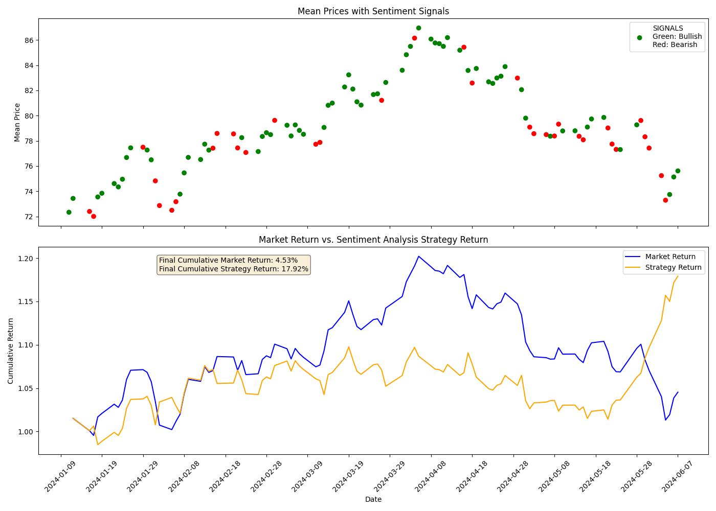
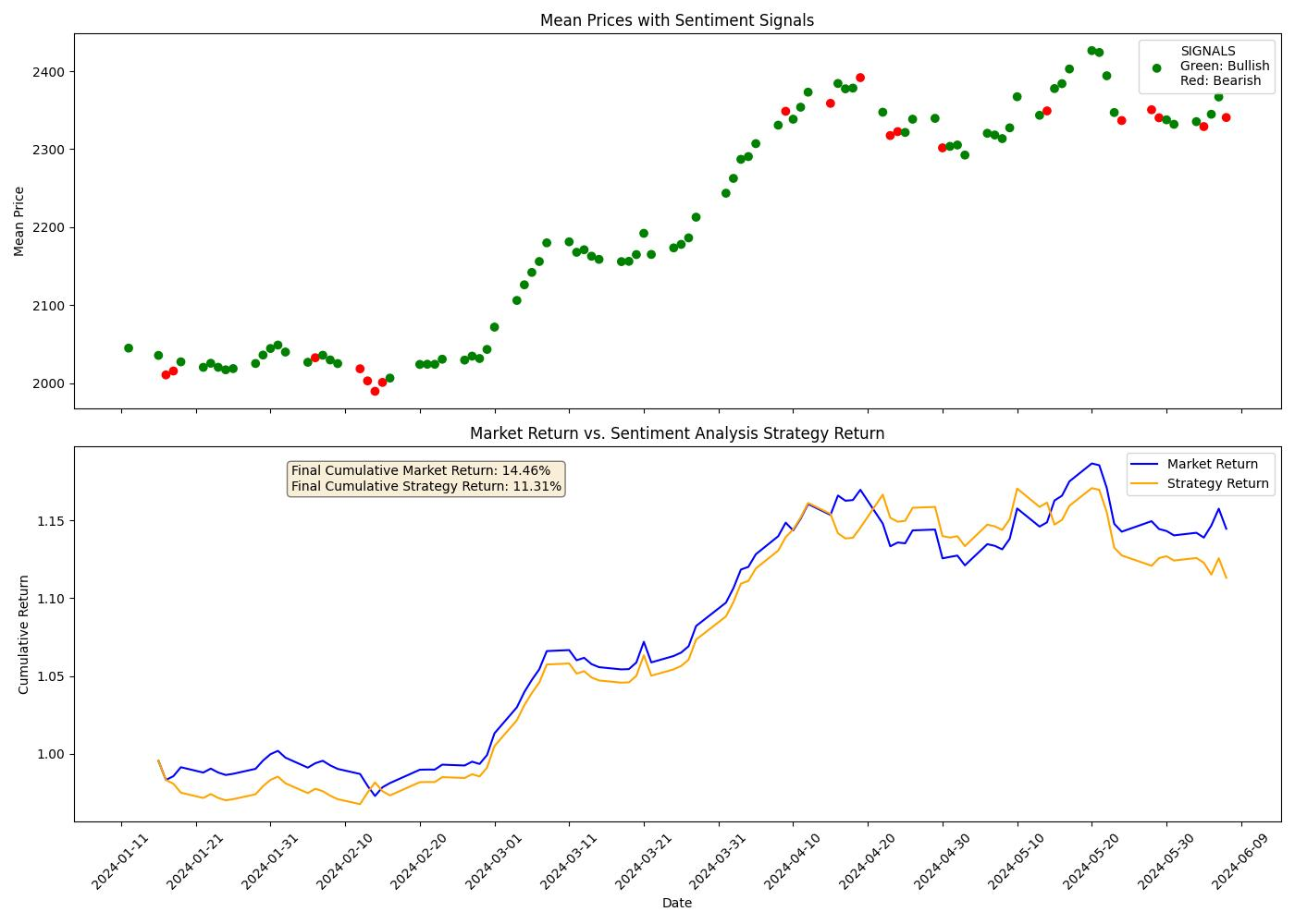
AWESOME! 资产新闻情感分析新工具

本段内容来自 AssetNewsSentimentAnalyzer 的使用说明

Asset News Sentiment Analyzer 最新发布到 0.1.4 版本，并加入到了 awesome-quant 推荐中。

一个简单的交易策略涉及来自该包的每日情绪分析信号，可以提供目标资产的基本市场吸引力（我们对过去 100 个市场日的商品进行了样本回测）。

这是原油的：

---

这是黄金的：

该Python库提供了两种复杂的工具，可通过 Google 搜索结果和在线新闻文章对金融资产和证券进行情感分析。您只需要一个 OpenAI API 密钥即可开始使用并利用此软件包提供的所有功能，即获取新闻文章、分析其内容并为投资和交易决策生成有见地的报告。

使用方法比较简单：

from asset_sentiment_analyzer import SentimentAnalyzer

# INITIALIZE THE ANALYZER
analyzer = SentimentAnalyzer(asset='Crude Oil', openai_key='your-openai-key')

# GET SENTIMENT ANALYSIS AS STRING FOR TODAY OR ANY DATE IN THE PAST (RETURNS "BULLISH", "BEARISH", OR "NEUTRAL")
sentiment = analyzer.get_sentiment(date='06-02-2024')
print(f"The sentiment for the asset is: {sentiment}")

# FETCH NEWS LINKS FOR ANY DATE WITH NEWS_DATE ARGUMENT IN MM-DD-YYYY FORMAT.
news_links = analyzer.fetch_news_links(news_date='06-02-2024')

# DISPLAY NEWS CONTENT
for url in news_links:
    print(analyzer.show_news_content(url))

# GENERATE A REPORT
report = analyzer.produce_daily_report(date='06-02-2024', max_words=300)
print(report)

---

你们都是在哪儿下载论文的？

上一期我们介绍了金融人最常看的顶刊。有同学问，要怎么订阅这些杂志。

其实答案只有一个，就是美金。它们的订阅地址在官网都有。

我知道我们都应该尊重知识产权。在我们的周刊里，到处是关于第三方知识产权的声明。不过，作为个人研究者，订阅所有的杂志、软件和书籍也是不太现实的。我通常的做法是，先看先用，如果确实有用且需要，我会去书店、电影院、官网加倍返还。

这里就介绍两个免费看论文的网站。第一个是 sci-hub。它已经保存了 25million 篇论文，索引压缩包就达 478M。搜索方式是按标题和按引用。

第二个网站是 freefullpdf,它的搜索使用了 google，搜索体验会更好一些。